The two fundamental mechanics to a vector search are:
- Retrieval Methods: these are algorithms used to efficiently find vectors, based on chosen distance metrics.
- Distance Metrics: used to determine and calculate vector “similarity”.
At a high-level, the process is:
- A provided query is converted to a vector, using the same embedding model as the vector database.
- The retrieval algorithm efficiently narrows down potential matches.
- The distance metric compares the
query vectorwithcandidate vectors. - Results are ranked, according to the distance metric’s concept of similarity.
- An arbitrary
knumber of ranked matches are then returned to the client.
Retrieval Methods
Retrieval algorithms are the methods used to efficiently find vectors within high-dimensional spaces, per the chosen distance metric. This process of identifying “neighbors” in a space, is called clustering.
 Credit: qdrant.tech
Retrieval methods can be dynamically changed at query time, without modifying the shape of vectors in a Vector Database. Each retrieval method however, will require it’s own distinct index data structure — hence, implementing more than one will mean parallel resource utilisation overhead.
The two common types of retrieval methods are:
K-nearest Neighbor (kNN)
This algorithm ensures the retrieval of the true number of nearest neighbors (k) for a given query vector. It does this by computing distances to every vector in that vector space — in this sense, it is often referred to as a “brute force search”.
- Due to the brute-forcing and thorough computations, it is best served in small to medium datasets (thousands to low millions of vectors).
- However, it provides perfect accuracy in captured neighbors.
- Index data structures are simplistic.
For tasks where the accuracy of each result is critical (such as in medical diagnosis or financial forecasting), kNN is probably your best bet, despite its higher computational demands.
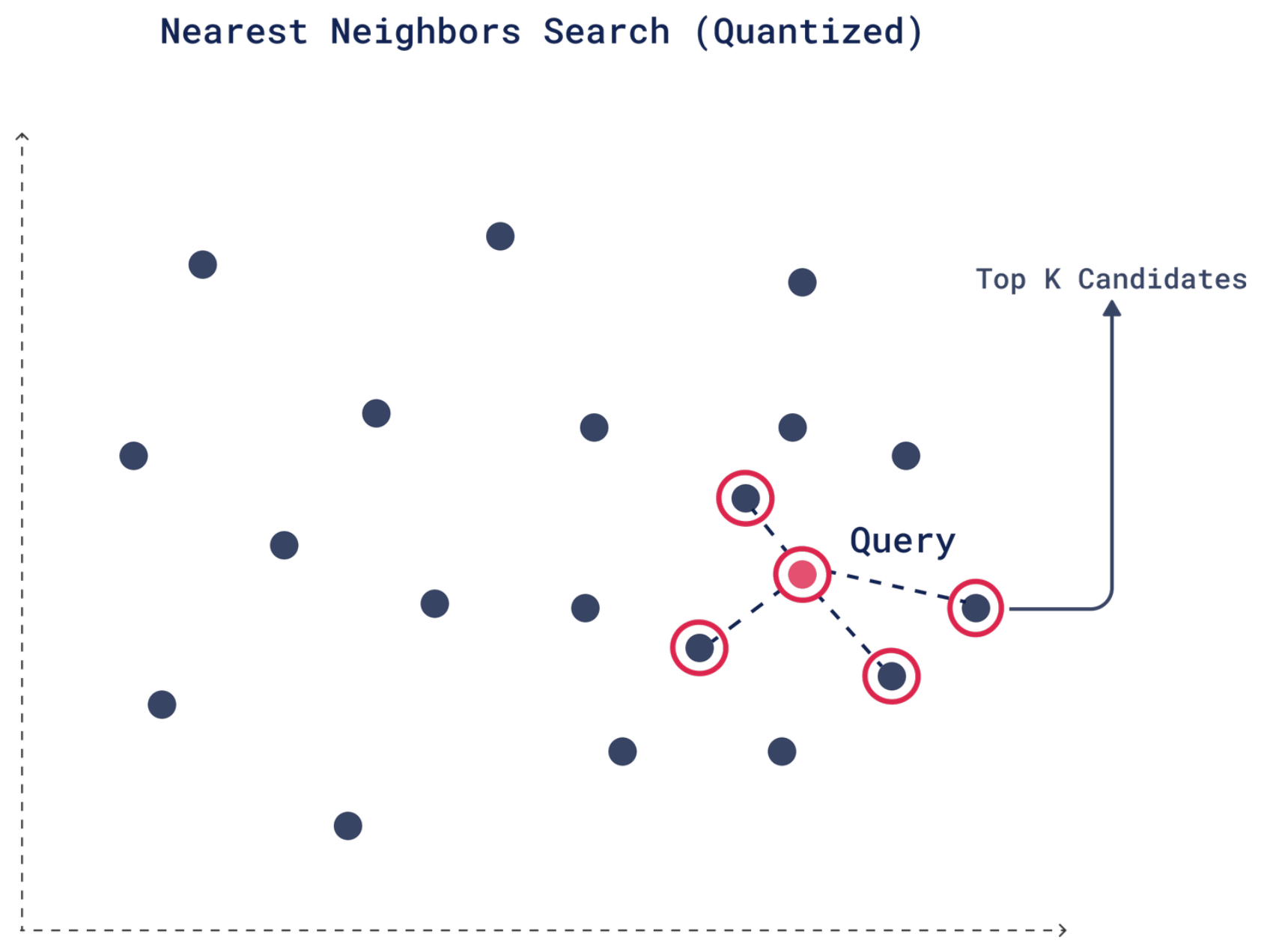
Approximate Nearest Neighbor Retrieval (aNN)
Approximate KNN algorithms sacrifice perfect accuracy for dramatic speed gains. It will return most, but not necessarily all of the true nearest neighbors — though the approximate nature can often be tuned to balance speed vs. accuracy.
- Due to it’s non-rigid context and approximating, aNN allows for rapid querying of even massive datasets in multi-dimensional space — without exponential requirement for computational resources.
In scenarios where speed and scalability are essential, especially when dealing with real-time searches in large databases (like search engines or recommendation systems), aNN makes more sense.
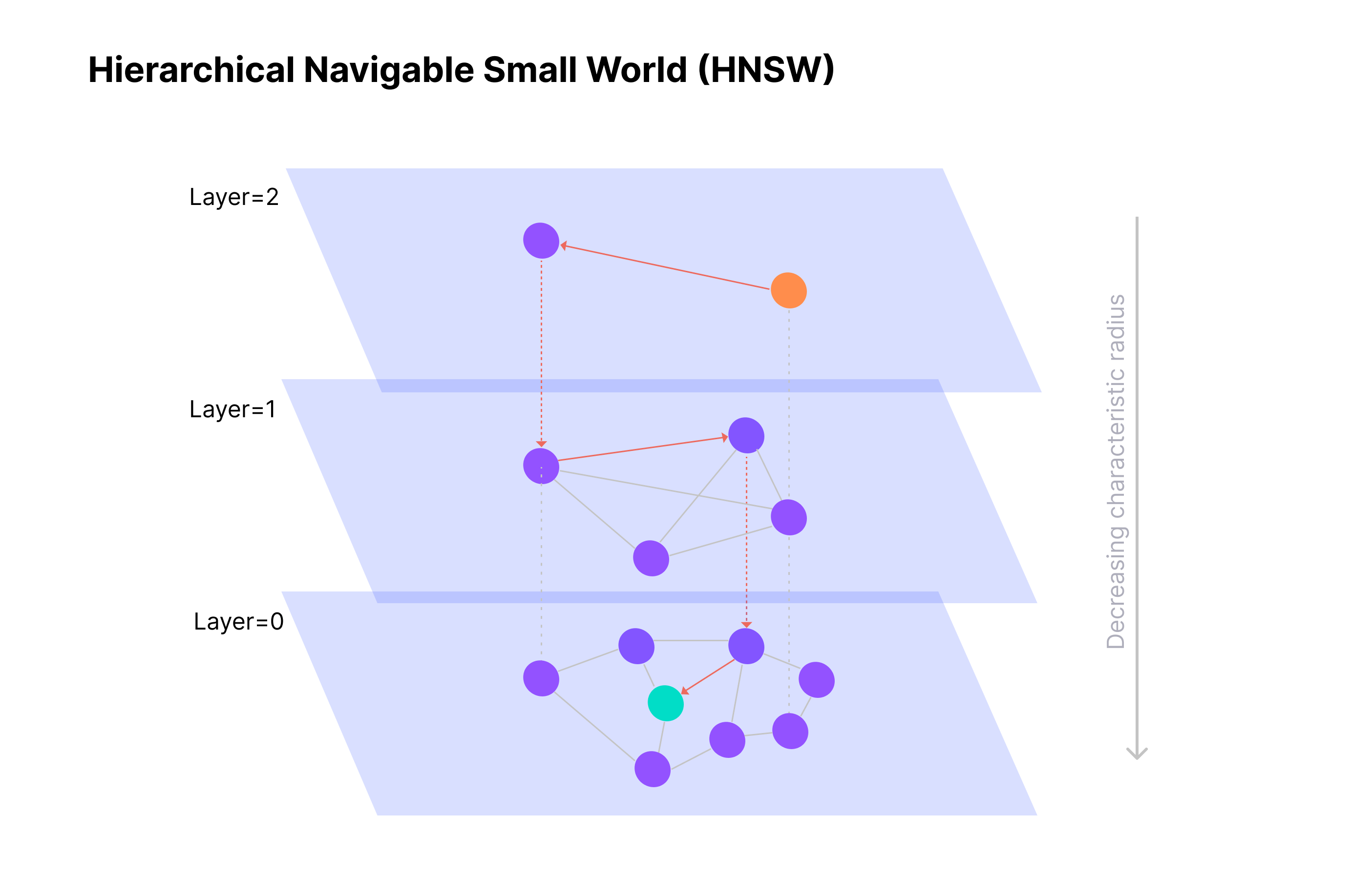
HNSW (Hierarchical Navigable Small Worlds)
HNSW is one of the most popular and effective approximate aNN algorithms used in modern vector databases. It allows excellent performance by creating a multi-layered graph structure that allows for efficient navigation through the vector space.
It achieves this through Skip Lists and Small World Properties (source).
 Credit: Zilliz.com
Small World Property:
A navigable small world graph is a network structure where most points, or “nodes,” are connected in a way that allows for efficient movement between any two points with only a few steps.
This characteristic, known as the “small world” property, means that even in large networks, it takes only a limited number of jumps to connect distant nodes.
Skip Lists:
A skip list is a layered data structure that speeds up searches by organizing information so that higher layers provide broad, approximate connections, while lower layers contain specific, detailed links. This layered setup allows searches to bypass unnecessary steps, “skipping” over parts of the dataset to hone in on relevant information quickly.
HNSW Summary:
At its core, HNSW creates a hierarchy of increasingly sparse graphs where each layer serves as a “navigation network” for the layer below it.
- By taking advantage of the structure’s gradation, higher layers can be used for rapid, coarse-grained exploration, while the finer, lower layers handle detailed searches.
- In this way, HNSW enables efficient, precise navigation through massive datasets.
This combination of coarse-to-fine search capability makes HNSW a powerful tool for complex, high-dimensional search tasks that traditional algorithms may struggle to perform.
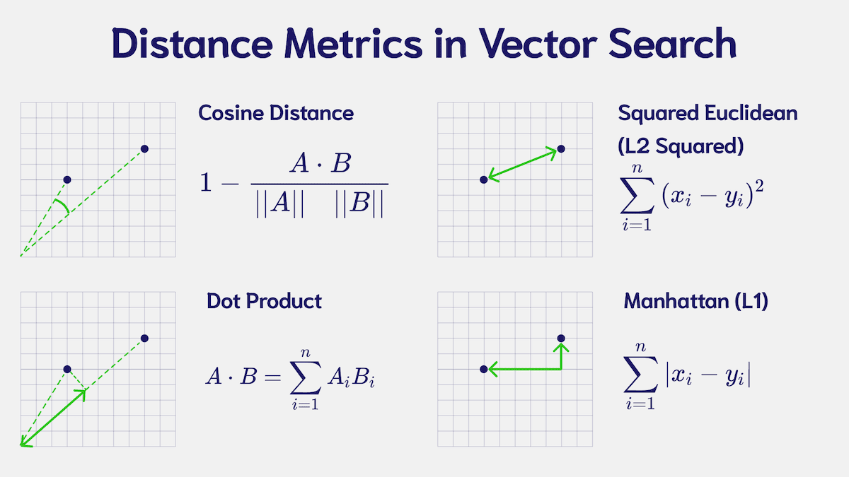
Distance Metrics
Distance metrics are rooted in the mathematical concepts of vectors and vector distance. Some commonly used methods to determine vector “distance” or “similarity” are below:
 Credit: Weaviate.io
High-level Overview of Common Distance Metrics:
| Metric | Description | Vector Properties Considered | Best Suited For |
|---|---|---|---|
| Euclidean Distance | Measures the straight-line distance between two points (or the hypotenuse). | Absolute position difference | Spatial data and clustering problems. It’s better for low-dimensional data and provides clear geometric interpretation, but loses accuracy in high-dimensional spaces. |
| Cosine Similarity | Calculates the cosine of the angle between two vectors. I.e the similarity of their angles, based on the point from which the angles meet. | Direction/orientation of the vectors | Text and semantic datasets where the vector direction is key. |
| Dot Product | Sums element-wise products of two vectors. The result is a single scalar value — not a vector array. | Combined magnitude and alignment | Ranking and relevance tasks, often used in recommendation systems. By incorporating magnitude, vectors can be considered the same topic, with the larger one being more “popular”. |
| Manhattan Distance | Sums the absolute differences of their coordinates. It is often referred to as the “Taxicab” distance since it mimics movement along blocks laid out in a grid. | Cumulative, absolute position difference. | Grid-based layouts and datasets where individual differences matter, such as pixel values (making it good for image recognition). It is often also used to identify outlier data points, as it is less sensitive to extreme values — this makes it a good candidate for anomaly detection systems. |
*The magnitude of a vector is its size. It can be calculated from the square root of the total of the squares of of the individual vector components.
- e.g
|V| = √(v₁² + v₂² + ... + vₙ²) - This allows for the effective factoring for of negative
floats, which is used within embeddings.